Linear Programming Code

All the code is written in matlab. Please visits here for a complete version of my code. The code base is in reference to Dr. Chunming Wang's MATH467 project code.

1. Implementation of the basic simplex algorithm

Code

    function [Solution,BasicVar,Status] = AxEqualsb(A, b, c, BasicVariables)
        [rows, ~] = size(b);
        if (all(b >= 0) && rank(A)==rows)
            [Solution,BasicVar,Status]=basicsimplex(A,b,c,BasicVariables);
        else
            disp('b must be nonnegative and rank(A) == size of b');
        end
    end

Interpretation

• The function works for Contraint $Ax=b$.
• It checks whether $b$ is non-nagative using all(b >= 0).
• It also checks the matrix $A$ is full rank using rank(A)==rows.
• If all the inputs are valid, we feed all the parameters into the basicsimplex() function and return the results.

Results

I use the following code to test the algorithm. I set A = [[1,0,1];[0,1,1]], b = [1;2], and c = [-1;-1;-3].
The result I expected to get is [0;1;1].

Running this to test:

    A = [[1,0,1];[0,1,1]];
    b = [1;2];
    c = [-1;-1;-3];
    
    [Solution,BasicVar,Status] = AxEqualsb(A, b, c, [1, 2])

Solution =

     0
     1
     1


BasicVar =

     3     2


Status =

     0

We can see the basic variables are $x_2$ and $x_3$ with values $1$ and $1$ respectively. Status = 0 showing the results are valid.

2. Implementation of general linear programming algorithm

Code

    function [Solution,BasicVar,Status] = AxSmallerThanb(A_hat, b_hat, c_hat)
        [rows, ~] = size(b_hat);
        if (all(b_hat >= 0) && rank(A_hat)==rows)
            I = eye(rows);
            c_new = [c_hat;zeros(rows,1)];
            A_new = [A_hat I];
            [~, A_cols] = size(A_hat);
            BasicVariables = (A_cols+1):(rows+A_cols);
            [Solution,BasicVar,Status]=basicsimplex(A_new,b_hat,c_new,BasicVariables);     
        else
            disp('b_hat must be nonnegative and rank(A) == size of b_hat');
        end
    end
    function [Solution,BasicVar,Status] = AxGreaterThanb(A_tilda, b_tilda, c_tilda)
        [rows, ~] = size(b_tilda);
        if (all(b_tilda >= 0) && rank(A_tilda)==rows)
            I = eye(rows);
            A_phaseII = [A_tilda -I];
            c_phaseII = [c_tilda;zeros(rows, 1)];
            A_phaseI = [A_phaseII I];
            [~, A_cols] = size(A_tilda);
            PhaseI_BasicVariables = (A_cols+1+rows):(2*rows+A_cols);
            c_phaseI = [zeros(A_cols+rows, 1);ones(rows, 1)];
            [SolutionI,BasicVarI,StatusI]=basicsimplex(A_phaseI,b_tilda,c_phaseI,PhaseI_BasicVariables);
            if (StatusI==0)
                % Phase II
                [Solution,BasicVar,Status]=basicsimplex(A_phaseII,b_tilda,c_phaseII,BasicVarI);
            else
                Solution=SolutionI;
                BasicVar=BasicVarI;
                Status=StatusI;
            end
        else
            disp('b_tilda must be nonnegative and rank(A) == size of b_tilda');
        end
    end

Interpretation

• The first function AxSmallerThanb() works for Contraint $Ax\leq b$.
  • It checks whether $b$ is non-nagative using all(b >= 0).
  • It also checks the matrix $A$ is full rank using rank(A)==rows.
  • If all the inputs are valid, we are going to add slack variables to make the problem standard.
  • Finally, we feed all the parameters into the basicsimplex() function and return the results.
• The second function AxGreaterThanb() works for Contraint $Ax\geq b$.
  • It checks whether $b$ is non-nagative using all(b >= 0).
  • It also checks the matrix $A$ is full rank using rank(A)==rows.
  • If all the inputs are valid, we are going to first add slack variables to make the problem standard, and call it A_phaseII.
  • Second, we are going to add phase I variables so that we have an intial basic solution.
  • Third, change the objective function based on the phase I variables .
  • Next, we feed all the parameters into the basicsimplex() function and return the results.
  • Then, do phase II simplex method based on the BasicVarI returned from phase I.
  • Finally, the results are returned.

Results

I'm going to use the same $A$, $b$, and $c$ as part 1.

Running this to test:

    [Solution,BasicVar,Status] = AxSmallerThanb(A, b, c)
    [Solution,BasicVar,Status] = AxGreaterThanb(A, b, c)

Solution =

     0
     1
     1
     0
     0


BasicVar =

     3     2


Status =

     0


Solution =

     0
     0
     2
     1
     0


BasicVar =

     4     3


Status =

    -1

• We can see for the first case, the basic variables are $x_2$ and $x_3$ with values $1$ and $1$ respectively. Status = 0 showing the results are valid.
• For the second case, it's straightforward that the solution will be infinity. Indeed, Status = -1 proves that there's no solution for this case.

3. Study of $L^1$ versus $L^2$ approximation

Code

    % Part 3 Apple stock vs Dow Jones Index
    Apple = readtable('APPL_DATA.csv');
    Apple = flipud(Apple);
    Apple = Apple(1:253,[1,4]);
    Apple = table2array(Apple(:,2));
    DowJones = readtable('Dow_Jones.csv');
    DowJones = DowJones(:,1:2);
    DowJones = table2array(DowJones(:,2));

    DowJones = str2double(DowJones);

    X = transpose(DowJones)
    Y = transpose(Apple)
    n = 253;

    % L1 Regression
    [RegressionModel]=L1_MultilinearRegression(X,Y);
    %
    % Least square
    %
    Xhat=X-mean(X,2)*ones(1,n);
    Yhat=Y-mean(Y);
    Coef_LSQ=inv(Xhat*Xhat')*Xhat*Yhat';
    Intersect_LSQ=mean(Y)-Coef_LSQ'*mean(X,2);
    Prediction=Coef_LSQ'*X+Intersect_LSQ;
    %
    figure;
    plot(Y,RegressionModel.Prediction,'o','MarkerSize',[8],'MarkerFaceColor','r','MarkerEdgeColor','r');
    hold on
    plot(Y,Prediction,'o','MarkerSize',[8],'MarkerFaceColor','b','MarkerEdgeColor','b');
    %
    figure;
    plot(Y'-RegressionModel.Prediction,'o','MarkerSize',[8],'MarkerFaceColor','r','MarkerEdgeColor','r');
    hold on
    plot(Y-Prediction,'o','MarkerSize',[8],'MarkerFaceColor','b','MarkerEdgeColor','b');

    RegressionModel.SRE
    sum(abs(Y-Prediction))

Explanation

• For this part of the problem, I'm using Apple Stock Price data and Dow Jones Index Price data for the past year.
• First, I read the data from the .csv files and do some manipulations to them to a vector.
• Second, I feed both data into L1_MultilinearRegression(X,Y), X is Dow Jones data and Y is Apple data. This should return a $L^1$ model.
• Third, I perform $L^2$ regression on the same set of data.
• Close to finish, I plot the regression model and the residual graph for both types of regression, shown in figures below.
• Finally, I return the sum of residuals for both models.

Results

Figure for regression model:

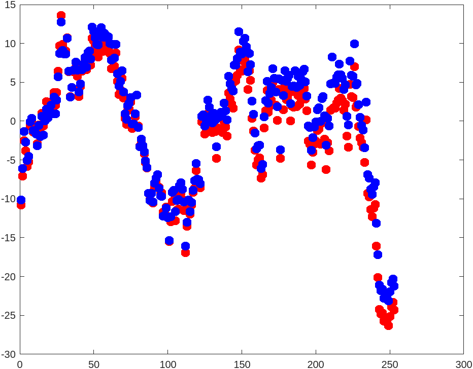
Figure for residual plot:

Sum of residuals (first one is for $L^1$, second one is for $L^2$):

ans =

   1.5284e+03


ans =

   1.5824e+03

Comparison of Results

The sum of $L^2$ residuals is a little higher than the sum of $L^1$ residuals. We also discover that $L^2$ typically guards against severe mistakes. The red dot in the picture above, which reflects $L^1$ predictions, is visible more frequently in areas farthest from $y=0$. This is due to the tendency of $L^2$ regression to punish extreme spots (projections represented in blue dot).